By Andrew Thompson

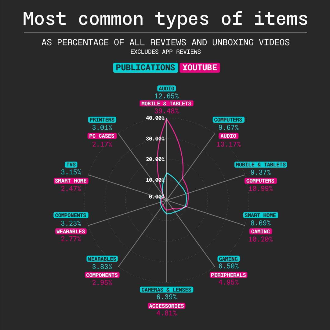
The Components report "The New Pornographers" examines the fetishism of tech reviewers for shiny, sexualized products over ones that are robust and functional. As we argued, manufacturers design objects not for use, but for imagery. This image primacy is illustrated in the enormous emphasis placed on mobile devices in YouTube tech reviews and unboxing videos, where, as we said, "the telegenic qualities of mobile devices work with the platform in a way that other objects, like laptops, headphones, and GPUs, can't leverage. In turn, not only do mobile devices dominate the mindshare of YouTube tech channels, but manufacturers design products with even more fanatical attention to how the product will present in such videos, further cementing the device's target audience not as users, but as viewers."

That colonization of attention is illustrated in the text's accompanying graph, which compares categories of products reviewed by print and web publications vs. those of YouTube tech influencers:

The challenge in arriving at these numbers is twofold. First, the four tech publications used in this analysis (PCMag, Trusted Reviews, Tech Radar, and CNET; see the dataset) do not all use the same categories for the same products. For example, here are the categories each of them uses for the Bose SoundSport:

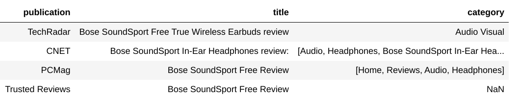
CNET and PCMag have hierarchies that are difficult to reconcile with one another, TechRadar uses the "Audio Visual" category that neither of the other three do, and Trusted Reviews has no category at all.

Second, categories on YouTube videos (dataset) are a cacophony of hashtags that vary from reviewer to reviewer who use them to game YouTube's algorithm rather than provide any sense of order. In order to look at both groups as a whole, and to compare them to one another, a single set of category tags has to be used across both corpora.

When analyzing these two datasets, I used K-Nearest Neighbors, the straightforward supervised algorithm that classifies vectors based on the classes of the n nearest. I'll walkthrough how I used PC Mag categories as the training data to classify all other articles, and then leveraged the classified articles on the text of YouTube videos to apply a standardized classification scheme to the entire dataset.

Tokenizing

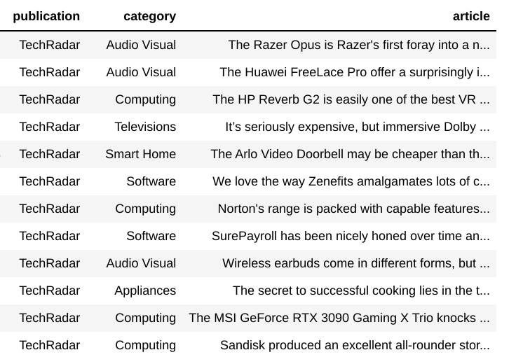
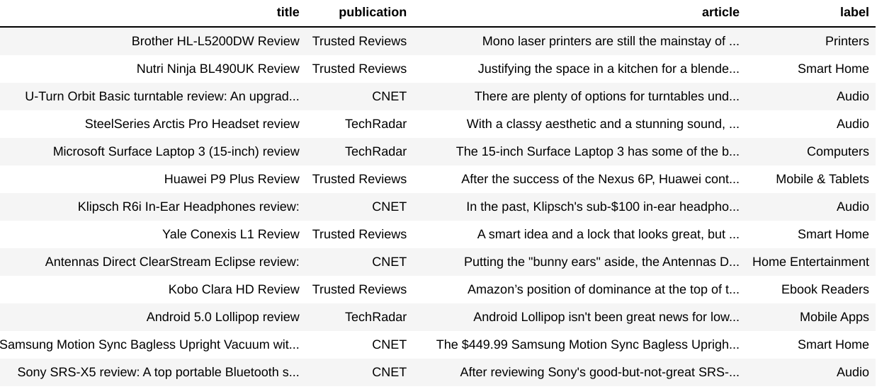
We can jump past the earliest preprocessing steps of basic cleaning and filtering and move straight to tokenizing the articles. Here's the head of our current dataframe, looking at just the publication, category and article columns:

For tokenization, we'll use Spacy. We'll first import Spacy's large English model:

import spacy
nlp = spacy.load('en_core_web_lg')

We'll create a new column on the dataframe, tokens, for the tokenized text. We'll also parallelize the tokenization process using the multiprocessing library to save time:

from multiprocessing import Pool

def tokenize(text):
    doc = nlp(text)
    return ' '.join(e.lemma_.lower() for e in doc)
    
def parallelize_dataframe(df, func, n_cores=4):
    df_split = np.array_split(df, n_cores)
    pool = Pool(n_cores)
    df = pd.concat(pool.map(func, df_split))
    pool.close()
    pool.join()
    return df

def return_df(df):
    df['tokens'] = df['article'].apply(tokenize)
    return df
    
df = parallelize_dataframe(df, return_df)    

Next, we'll get rid of anything that isn't an alphabetic character — as numbers and punctuation create meaningless noise in our classification — and we'll reduce multiple whitespace characters to a single characters. We'll also get rid of any rows that are missing data:

df['tokens'] = df['tokens'].apply(lambda x: re.sub(r'[^a-zA-Z ]', ' ', x))
df['tokens'] = df['tokens'].apply(lambda x: re.sub(r' {1,}', ' ', x))

df = df[~df['tokens'].apply(lambda x: isinstance(x, float))]

Now we'll count every token in the dataset so that we can create less noisy document vectors. Ultimately, we'll only want tokens that are in the 90th percentile (to remove relatively unusual words that can misclassify), and tokens that are not greater than the 99.9th percentile (to remove domain-specific stopwords that Spacy may not recognize):

from collections import Counter

word_counter = Counter()

for tokens in df['tokens']:
    for word in tokens.split():
        word_counter[word] += 1

##create new df with all the words

vocab = pd.DataFrame(columns = ['word', 'count'])
vocab['count'] = pd.Series(list(word_counter.values()))
vocab['word'] = pd.Series(list(word_counter.keys()))
vocab.index = vocab['word']

del vocab['word']

Vectorization and dimensionality reduction

With tokenization complete, we can vectorize the articles using TFIDF. While TFIDF is designed to down weight both stop words and words that don't appear frequently in a corpus, it doesn't do so perfectly, and it usually needs assistance from further filtering. Therefore, we'll only vectorize words that fit our 90th - 99.9th quantile parameters.

from sklearn.feature_extraction.text import TfidfVectorizer

upper_quantile = .999
lower_quantile = .9

#getting only words from the vocab list between the two quantile ranges
vecvocab = list(vocab[(vocab['count'] < vocab['count'].quantile(upper_quantile)) &
                       (vocab['count'] > vocab['count'].quantile(lower_quantile))].index)

#loading the spacy stop words list
spacy_stop_words = list(nlp.Defaults.stop_words)

tfidf = TfidfVectorizer(vocabulary=vecvocab, stop_words=spacy_stop_words, tokenizer=None)

#creating the vector matrix of tokens
vec_matrix = tfidf.fit_transform(df['tokens'])

We'll perform dimensionality reduction with TruncatedSVD down to 200 dimensions to get our vec_matrix that we'll use to train our classifier:

from sklearn.decomposition import TruncatedSVD

pca = TruncatedSVD(n_components=200)
vec_matrix = pca.fit_transform(vec_matrix)

Creating training labels

Before we can train, we need the PCMag labels. Of the four publications studied in the report, PCMag had the most reliably useful categories: The third subcategories in its taxonomy trees were the least likely to be overly specific (like a product name that would only apply to that review), or overly broad (like "Audio Visual"). For example, in two products whose taxonomies include[Home, Reviews, Audio, Headphones] and [Home, Reviews, Audio, Speakers], we just want the Audio value so that they can be group together.

We'll first get rid of all the null values in the category column:

df['category'].fillna('None', inplace=True)

First we'll grab all the PCMag reviews and remove the ones that don't have a third value, and then create a column with categories from that third value:

pcmag = df[(df['publication'] == 'PCMag') & (df['category'] != 'None')]
pcmag = pcmag[pcmag['category'].apply(lambda x: len(x) > 2)]

pcmag['third_cat'] = pcmag['category'].apply(lambda x: x[2])

This gives us a total of the following 50 categories:

array(['Mobile Apps', 'Audio', 'Games', 'Cars & Auto',
       'Subscription Services', 'Operations', 'Health & Fitness',
       'Printers', 'Projectors', 'Productivity', 'Gaming Hardware',
       'Website & App Building Tools', 'Music & Audio', 'Accounting',
       'Photo & Design', 'VR', 'Laptops', 'Desktop PCs', 'Tablets',
       'Monitors', 'Input Devices', 'Networking', 'Storage',
       'Communications', 'IT Management', 'Video', 'Sales & Marketing',
       'Smart Home', 'Scanners', 'Mobile Phones', 'Security',
       'System Utilities', 'Tech for Kids', 'Home Entertainment',
       'Ebook Readers', 'Digital Life', 'Shredders', 'Components',
       'Education', 'Batteries & Power', 'Operating Systems', 'Wearables',
       'Human Resources', 'Cameras', 'IT Security', 'Personal Finance',
       'Video Cameras', 'E-Commerce & Payments', 'Data Analytics',
       'Drones'], dtype=object)

Many of these are software and apps that we'll later ignore. But a few can arguably further consolidated. "Mobile Phones" and "Tablets" can be lumped into a single "Mobile & Tablets", while "Desktop PCs" and "Laptops" can be brought into a single "Computers" category. Watches are sometimes thrown into the "Wearables" category and sometimes into "Health & Fitness"; we'll regularize it by making sure it's always in the former. Others can be renamed, like changing "Input Devices" into "Peripherals."

So we can do a quick cleanup. Although a stack of lambda functions is slower and substantially uglier than a single function, its presentation is more modular and, at least for me, easier to work with:

pcmag['third_cat'] = pcmag['third_cat'].apply(lambda x: 'Mobile & Tablets' if 'Mobile Phones' in x or 'Tablets' in x else x)
pcmag['third_cat'] = pcmag['third_cat'].apply(lambda x: 'Gaming' if 'Games' in x or 'Gaming' in x else x)
pcmag['third_cat'] = pcmag['third_cat'].apply(lambda x: 'Cameras & Lenses' if 'Cameras' in x or 'Lenses' in x else x)
pcmag['third_cat'] = pcmag['third_cat'].apply(lambda x: 'Peripherals' if x == 'Input Devices' else x)
pcmag['third_cat'] = pcmag['third_cat'].apply(lambda x: 'Components' if x == 'Components' or x == 'Storage' else x)
pcmag['third_cat'] = pcmag['third_cat'].apply(lambda x: 'Computers' if x == 'Laptops' or x == 'Desktop PCs' else x)
pcmag['third_cat'] = pcmag['third_cat'].apply(lambda x: 'Wearables' if 'Watch' in x else x)

(Note: The version of the graph pictured above relied on a somewhat different set of re-categorization steps, which accounts for a few differently named categories, as well as the slight differences in proportional values.)

Cross-validating

We'll first do a few cross-validation runs to see how many neighbors our KNN classifier should use. We'll make our cleaned PCMag labels into a single list that we can pass to the KNN classifier, and we'll grab the index values of just the PCMag vectors from our token matrix:

pcmag_index = pcmag.index  
labels = list(pcmag['third_cat'])

We'll set a minimum neighbor value of 1 and a max neighbor value of 7. We'll also use the weights distance metric in our classifier so that closer neighbors are upweighted and farther neighbors downweighted:

from sklearn.neighbors import KNeighborsClassifier

#creating a dataframe to save the results of the validation runs
testing_df = pd.DataFrame(index = [i for i in range(0,30)], 
                          columns=[e for e in range(1,7)])

#testing from 30 different seeds
for seed in range(0,30):
    from sklearn.model_selection import train_test_split

    X = vec_matrix[pcmag_index]
    y = labels
    X_train, X_test, y_train, y_test = train_test_split(
        X, y, test_size=0.2, random_state=seed)
    
    for neighbor_number in range(1, 7):
        clf = KNeighborsClassifier(n_neighbors=neighbor_number,
        weights='distance').fit(X_train, y_train)
        
        score = clf.score(X_test, y_test)
        testing_df.loc[seed, neighbor_number] = score

Based on our 30 cross-validation runs, we can get about 93% accuracy, which is highest and most frequently at the four-neighbor level:

               1           2          3        4           5           6
is_max         4           4          8       13           4           4
mean    0.926926    0.926926    0.92938 0.930346    0.929091    0.928759

For our purposes, and for using such a straightforward out-of-the-box method, this is pretty good. This level of accuracy isn't high enough to automate a passenger jet, but for understanding the basic contours of tech reviewers' interests — and for identifying a phenomenon like the large chasm of smartphone obsession that divides YouTuber influencers and their forebearers — it's perfectly acceptable.

Fitting the model

We'll set our n_neighbors value to 4 and fit the model on the PCMag labels:

knn = KNeighborsClassifier(n_neighbors=4, weights='distance')
knn.fit(vec_matrix[pcmag_index], labels)

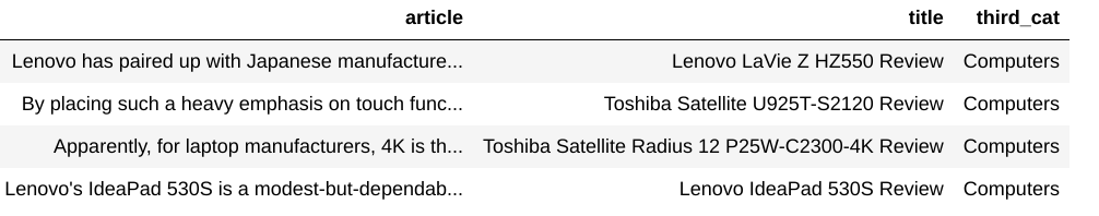
We can see the model in action by predicting individual rows. Here it predicts the class of a TechRadar review for a laptop:

In: 
product_row = 5000
print (df.loc[product_row]['title'])
print (df.loc[product_row, 'publication'])
print ('Predicted class:', knn.predict([vec_matrix[product_row]]))
print ('Labels:', knn.predict_proba([vec_matrix[product_row]]))

Out:
Toshiba Kira (2015) review
TechRadar
['Computers']
[[0. 0. 0. 0. 0. 0. 0. 1. 0. 0. 0. 0. 0. 0. 0. 0. 0. 0. 0. 0. 0. 0. 0. 0. 0. 0. 0. 0. 0.     0. 0. 0. 0. 0. 0. 0. 0. 0. 0. 0. 0. 0. 0. 0. 0.]]

The array of knn.predict_proba is the probability score of a class based on the combination of the classes of the four nearest neighbors and their weights. The array gives a 100% probability to one class — we can use knn.kneighbors to see which PCMag articles were responsible for the classification of the TechRadar laptop review:

Classifying and filtering by probability scores

So, after fitting, we just need to apply the model to our non-training data comprising the other publications:

df['label'] = list(map(knn.predict, [[e] for e in vec_matrix]))
df['label'] = df['label'].apply(lambda x: x[0]) #extracting the string value from the classified label

And it's done! We've standardized the entire tech review publication corpus:

Classifying YouTube reviews

Classifying the YouTube reviews involves re-training the KNN classifier on the entire now-classified publication corpus. It requires essentially the same previous steps, except that a combination of both a video's subtitles and description are tokenized and used for classification. Because the process is mostly redundant with everything that preceded, we won't go through it again here.

Conclusion

KNN out-of-the-box with sklearn provided a mostly uncomplicated, resourceful way to reconcile the categories among the corpora. Its ease of use and limited customizability comes with limitations, and if our report hinged on microscopic distinctions among product category prevalence, it would probably be insufficient. Luckily, the principle trend serviced by the graph — the disparity between the two media types in their fixation on mobile tech — was not microscopic, it was large and unmistakable, and vanilla KNN is helpful in identifying its general existence, even if its precise details may wiggle around with shifting parameters. Even a primitive machine learning algorithm is sensitive to YouTube's sexual obsession with the smartphone, something that, all data aside, is in any case glaringly apparent to anyone observing tech media today.